Introduction
The examples are from [this] textbook, and my class notes are [here].
Example 5.1 : The Electric Utility Data
An electric utility company is interested in developing a model relating peak-hour demand \((y)\) to total energy usage during the month \((x)\).
# load data
ex51 = read.table("ex5-1.txt",header = T)
head(ex51)
## Customer x_.kWh. y_.kW.
## 1 1 679 0.79
## 2 2 292 0.44
## 3 3 1012 0.56
## 4 4 493 0.79
## 5 5 582 2.70
## 6 6 1156 3.64# plot
plot(ex51$x_.kWh.,
ex51$y_.kW.,
xlab = "Usage",
ylab = "Demand")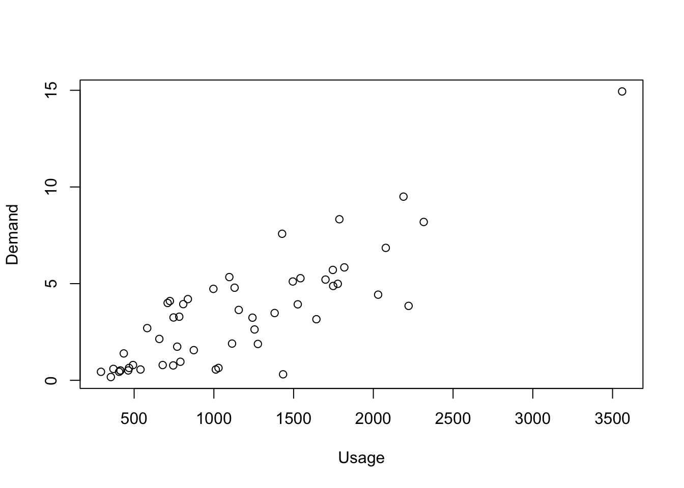
Figure 1: Scatter diagram of the energy demand (kW) versus energy usage (kWh)
As a starting point a simple linear regression model is assumed, and the least-squares fit is :
\[\hat y=-0.83130+0.00368x\]
# model
lm51 <- lm(ex51$y_.kW. ~ ex51$x_.kWh., data = ex51)
# summary (analysis of variance)
summary(lm51)
##
## Call:
## lm(formula = ex51$y_.kW. ~ ex51$x_.kWh., data = ex51)
##
## Residuals:
## Min 1Q Median 3Q Max
## -4.1399 -0.8275 -0.1934 1.2376 3.1522
##
## Coefficients:
## Estimate Std. Error t value Pr(>|t|)
## (Intercept) -0.8313037 0.4416121 -1.882 0.0655 .
## ex51$x_.kWh. 0.0036828 0.0003339 11.030 4.11e-15 ***
## ---
## Signif. codes: 0 '***' 0.001 '**' 0.01 '*' 0.05 '.' 0.1 ' ' 1
##
## Residual standard error: 1.577 on 51 degrees of freedom
## Multiple R-squared: 0.7046, Adjusted R-squared: 0.6988
## F-statistic: 121.7 on 1 and 51 DF, p-value: 4.106e-15# plot
plot(ex51$x_.kWh.,
ex51$y_.kW.,
xlab = "Usage",
ylab = "Demand")
abline(lm51, col = "red")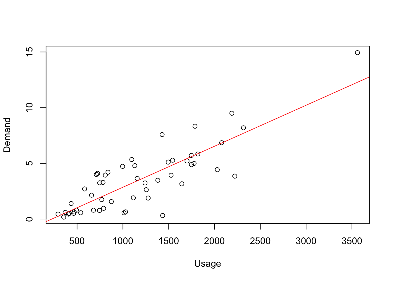
Figure 2: Scatter diagram of the energy demand (kW) versus energy usage (kWh) with Simple Linear Model
For this model \(R^2=0.7046\); that is about 70% of the variability in demand is accounted for by the straight-line fit to energy usage. The summary statistics do not reveal any obvious problems with this model.
# R-student values versus fitter values fitted
plot(fitted(lm51),
     rstudent(lm51),
     ylab=TeX(r'($t_i$)'),
     xlab=TeX(r'($\hat{y}_i$)'),
     pch = 16);abline(0, 0,lty = 2)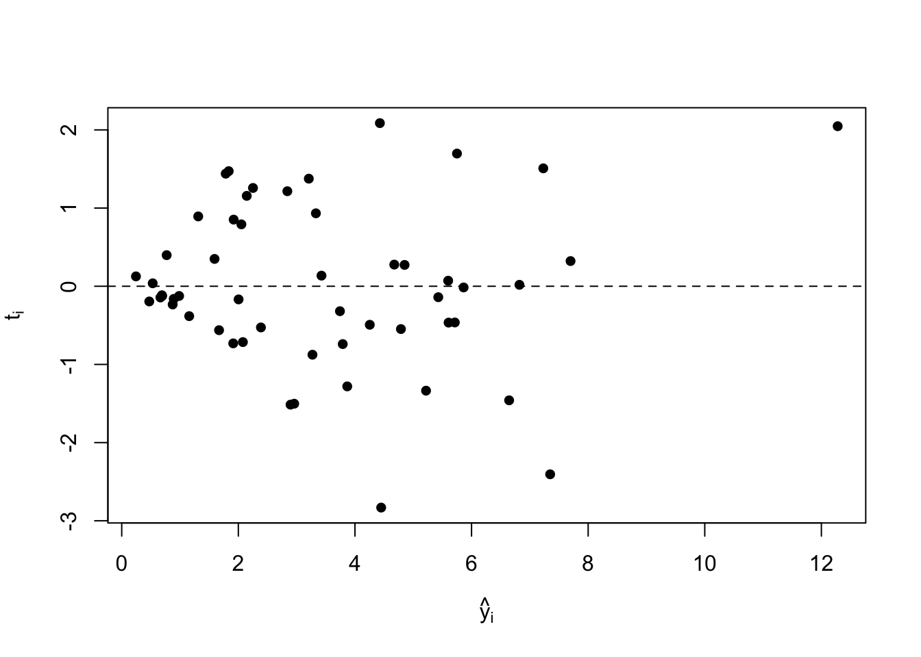
Figure 3: Plot of R-Student v.s fitted values
Residuals form an outward-opening funnel, indicating that the error variance is increasing as energy consumption increases. A transformation may be helpful helpful in correcting this model inadequacy. To select the form of the transformation, note that the response variable y may be viewed as a “count” of the number of kilowatts used by a customer during a particular hour. The simplest probabilistic model for count data is the Poisson distribution. This suggests regressing \(y^*=\sqrt{y}\) on x as a variance-stabilizing transformation. The resulting least-squares fit is :
\[\hat y^*=0.5822+0.0009529x\]
# y star
ex51$ystar <- sqrt(ex51$y_.kW.)
# transformed model
lm51T <- lm(ex51$ystar ~ ex51$x_.kWh., data = ex51)# summary (analysis of variance)
summary(lm51T)
##
## Call:
## lm(formula = ex51$ystar ~ ex51$x_.kWh., data = ex51)
##
## Residuals:
## Min 1Q Median 3Q Max
## -1.39185 -0.30576 -0.03875 0.25378 0.81027
##
## Coefficients:
## Estimate Std. Error t value Pr(>|t|)
## (Intercept) 5.822e-01 1.299e-01 4.481 4.22e-05 ***
## ex51$x_.kWh. 9.529e-04 9.824e-05 9.699 3.61e-13 ***
## ---
## Signif. codes: 0 '***' 0.001 '**' 0.01 '*' 0.05 '.' 0.1 ' ' 1
##
## Residual standard error: 0.464 on 51 degrees of freedom
## Multiple R-squared: 0.6485, Adjusted R-squared: 0.6416
## F-statistic: 94.08 on 1 and 51 DF, p-value: 3.614e-13# R-student values versus fitted values for the transformed data
plot(fitted(lm51T),
rstudent(lm51T),
ylab=TeX(r'($t_i$)'),
xlab=TeX(r'($\hat{y}^*_i$)'),
pch = 16);abline(0, 0,lty = 2)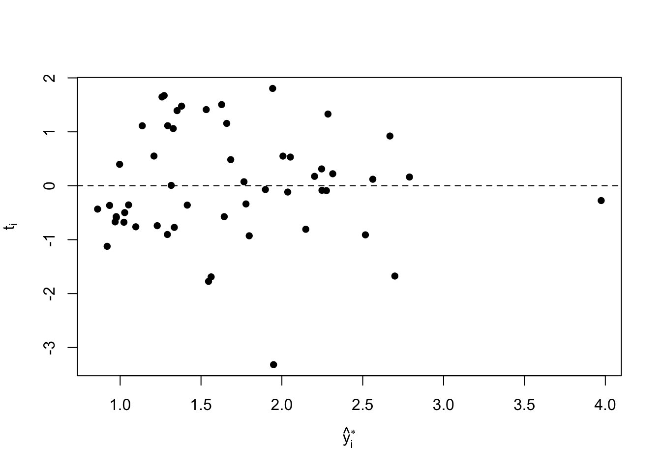
Figure 4: Plot of R-student values versus fitted values for the transformed data
The impression from examining this plot is that the variance is stable; consequently, we conclude that the transformed model is adequate.
Note that there is one suspiciously large residual (customer 26) and one customer whose energy usage is somewhat large (customer 50). The effect of these two points on the fit should be studied further before the model is released for use.
Example 5.2 : The Windmill Data
A research engineer is investigating the use of a windmill to generate electricity. He has collected data on the DC Output from his windmill and the corresponding wind velocity. The data are plotted in the table and Figure 5 below.
# load data
ex52 <- read.table("ex5-2.txt",header = T)
head(ex52)
## ObservationNumber_i WindVelocity_xi_mph DCOutput_yi
## 1 1 5.0 1.582
## 2 2 6.0 1.822
## 3 3 3.4 1.057
## 4 4 2.7 0.500
## 5 5 10.0 2.236
## 6 6 9.7 2.386# plot
plot(ex52$WindVelocity_xi_mph,
ex52$DCOutput_yi,
xlab = "Wind Velocity, x",
ylab = "DC Output, Y")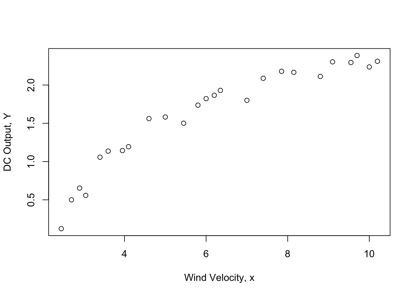
Figure 5: Plot of DC Output wind velocity x for the windmill data
Inspection of the scatter diagram indicates that the relationship between DC output \((y)\) and wind velocity \((x)\) may be nonlinear. However, we initially fit a straight-line model to the data. The regression model is :
\[\hat y=0.1309+0.2411x\]
# model
lm52 <- lm(ex52$DCOutput_yi ~ ex52$WindVelocity_xi_mph, data = ex52)
# plot
plot(ex52$WindVelocity_xi_mph,
     ex52$DCOutput_yi,
     xlab = "Wind Velocity, x",
     ylab = "DC Output, Y")
abline(lm52, col = "red")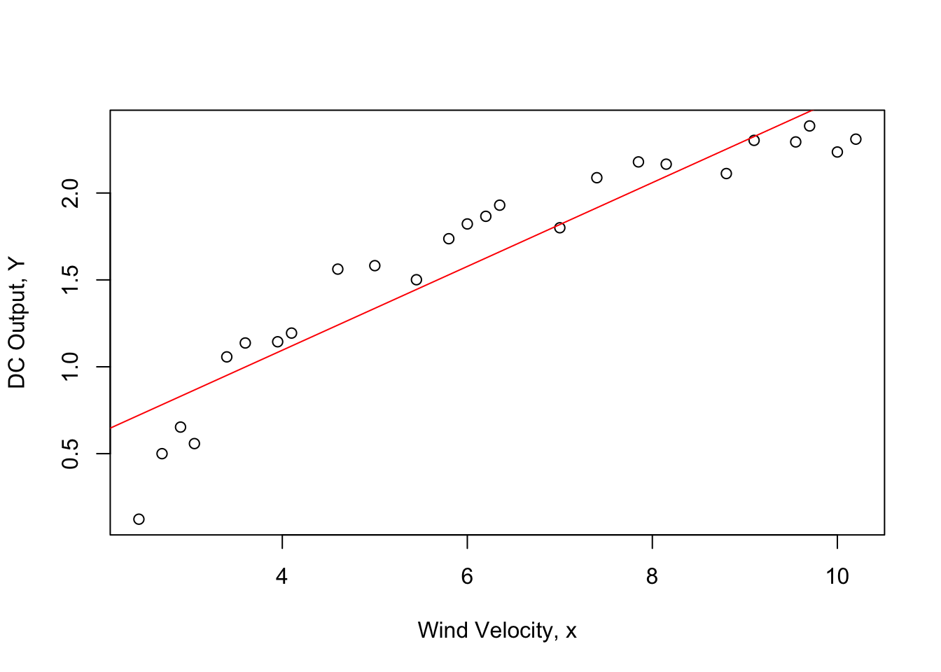
Figure 6: Plot of DC Output wind velocity x for the windmill data with SLM
# summary (analysis of variance)
summary(lm52)
##
## Call:
## lm(formula = ex52$DCOutput_yi ~ ex52$WindVelocity_xi_mph, data = ex52)
##
## Residuals:
## Min 1Q Median 3Q Max
## -0.59869 -0.14099 0.06059 0.17262 0.32184
##
## Coefficients:
## Estimate Std. Error t value Pr(>|t|)
## (Intercept) 0.13088 0.12599 1.039 0.31
## ex52$WindVelocity_xi_mph 0.24115 0.01905 12.659 7.55e-12 ***
## ---
## Signif. codes: 0 '***' 0.001 '**' 0.01 '*' 0.05 '.' 0.1 ' ' 1
##
## Residual standard error: 0.2361 on 23 degrees of freedom
## Multiple R-squared: 0.8745, Adjusted R-squared: 0.869
## F-statistic: 160.3 on 1 and 23 DF, p-value: 7.546e-12# MSE <- c(crossprod(resid(lm52)))/length(resid(lm52));MSEThe summary statistics for this model are \(R^2=0.8745\), and \(F_0=160.26\) (the P-value is <0.0001).
# yhat and e
ex52$fitted <- fitted(lm52)
ex52$resid <- resid(lm52)
ex52 %>% arrange(-desc(ex52$WindVelocity_xi_mph))
## ObservationNumber_i WindVelocity_xi_mph DCOutput_yi fitted resid
## 1 25 2.45 0.123 0.7216899 -0.59868986
## 2 4 2.70 0.500 0.7819771 -0.28197708
## 3 11 2.90 0.653 0.8302069 -0.17720685
## 4 8 3.05 0.558 0.8663792 -0.30837918
## 5 3 3.40 1.057 0.9507813 0.10621871
## 6 16 3.60 1.137 0.9990111 0.13798894
## 7 24 3.95 1.144 1.0834132 0.06058683
## 8 23 4.10 1.194 1.1195855 0.07441450
## 9 13 4.60 1.562 1.2401599 0.32184007
## 10 1 5.00 1.582 1.3366195 0.24538052
## 11 20 5.45 1.501 1.4451365 0.05586353
## 12 14 5.80 1.737 1.5295386 0.20746142
## 13 2 6.00 1.822 1.5777683 0.24423165
## 14 10 6.20 1.866 1.6259981 0.24000188
## 15 12 6.35 1.930 1.6621705 0.26782955
## 16 19 7.00 1.800 1.8189172 -0.01891722
## 17 15 7.40 2.088 1.9153768 0.17262323
## 18 17 7.85 2.179 2.0238938 0.15510624
## 19 9 8.15 2.166 2.0962384 0.06976158
## 20 18 8.80 2.112 2.2529852 -0.14098518
## 21 21 9.10 2.303 2.3253298 -0.02232985
## 22 7 9.55 2.294 2.4338468 -0.13984684
## 23 6 9.70 2.386 2.4700192 -0.08401917
## 24 5 10.00 2.236 2.5423638 -0.30636383
## 25 22 10.20 2.310 2.5905936 -0.28059360The observations are arranged in order of increasing wind speed. The residuals show a distinct pattern, that is, they move systematically from negative to positive and back to negative again as wind speed increases.
# plot
plot(fitted(lm52),
     resid(lm52),
     ylab=TeX(r'($e_i$)'),
     xlab=TeX(r'($\hat{y}_i$)'),
     pch = 16);abline(0, 0,lty = 2)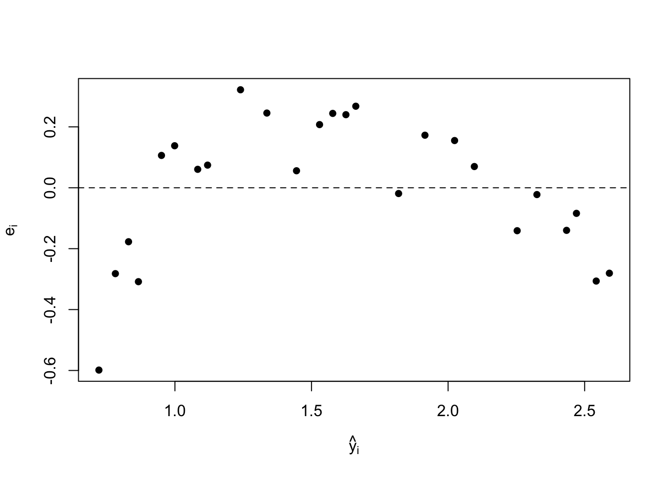
This residual plot indicates model inadequacy and implies that the linear relationship has not captured all of the information in the wind speed variable. Note that the curvature was apparent in the earlier scatter diagram, is greatly amplified in the residual plot.
Clearly some other model form must be considered. We might initially consider using a quadratic model such as :
\[y=\beta_0+\beta_1x+\beta_2x^2+\epsilon\]
to account for the curvature. However since the quadratic model will eventually bend downward as wind speed increases, it would not be appropriate for these data. A more reasonable model for windmill data that incorporates an upper asymptote would be :
\[y=\beta_0+\beta_1(\frac{1}{x})+\epsilon\]
# transformation
ex52$xstar <- 1/ex52$WindVelocity_xi_mph
# transformed model
lm52T <- lm(ex52$DCOutput_yi ~ ex52$xstar, data = ex52)
# transformaion summary
summary(lm52T)
##
## Call:
## lm(formula = ex52$DCOutput_yi ~ ex52$xstar, data = ex52)
##
## Residuals:
## Min 1Q Median 3Q Max
## -0.20547 -0.04940 0.01100 0.08352 0.12204
##
## Coefficients:
## Estimate Std. Error t value Pr(>|t|)
## (Intercept) 2.9789 0.0449 66.34 <2e-16 ***
## ex52$xstar -6.9345 0.2064 -33.59 <2e-16 ***
## ---
## Signif. codes: 0 '***' 0.001 '**' 0.01 '*' 0.05 '.' 0.1 ' ' 1
##
## Residual standard error: 0.09417 on 23 degrees of freedom
## Multiple R-squared: 0.98, Adjusted R-squared: 0.9792
## F-statistic: 1128 on 1 and 23 DF, p-value: < 2.2e-16The fitted regression model is \[\hat y=2.9789-6.9345x'\]
The summary statistics for this model are\(R^2=0.98\), and \(F_0=1128\) (the p value is <0.0001).
# R-student values versus fitted values for the transformed data
plot(fitted(lm52T),
     rstudent(lm52T),
     ylab=TeX(r'($t_i$)'),
     xlab=TeX(r'($\hat{y}_i$)'),
     pch = 16);abline(0, 0,lty = 2)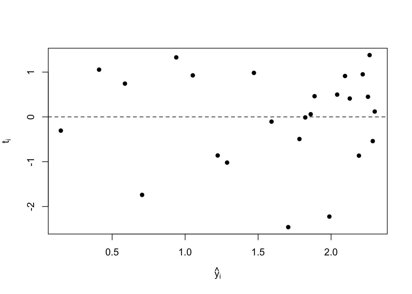
This plot does not reveal any serious problems.
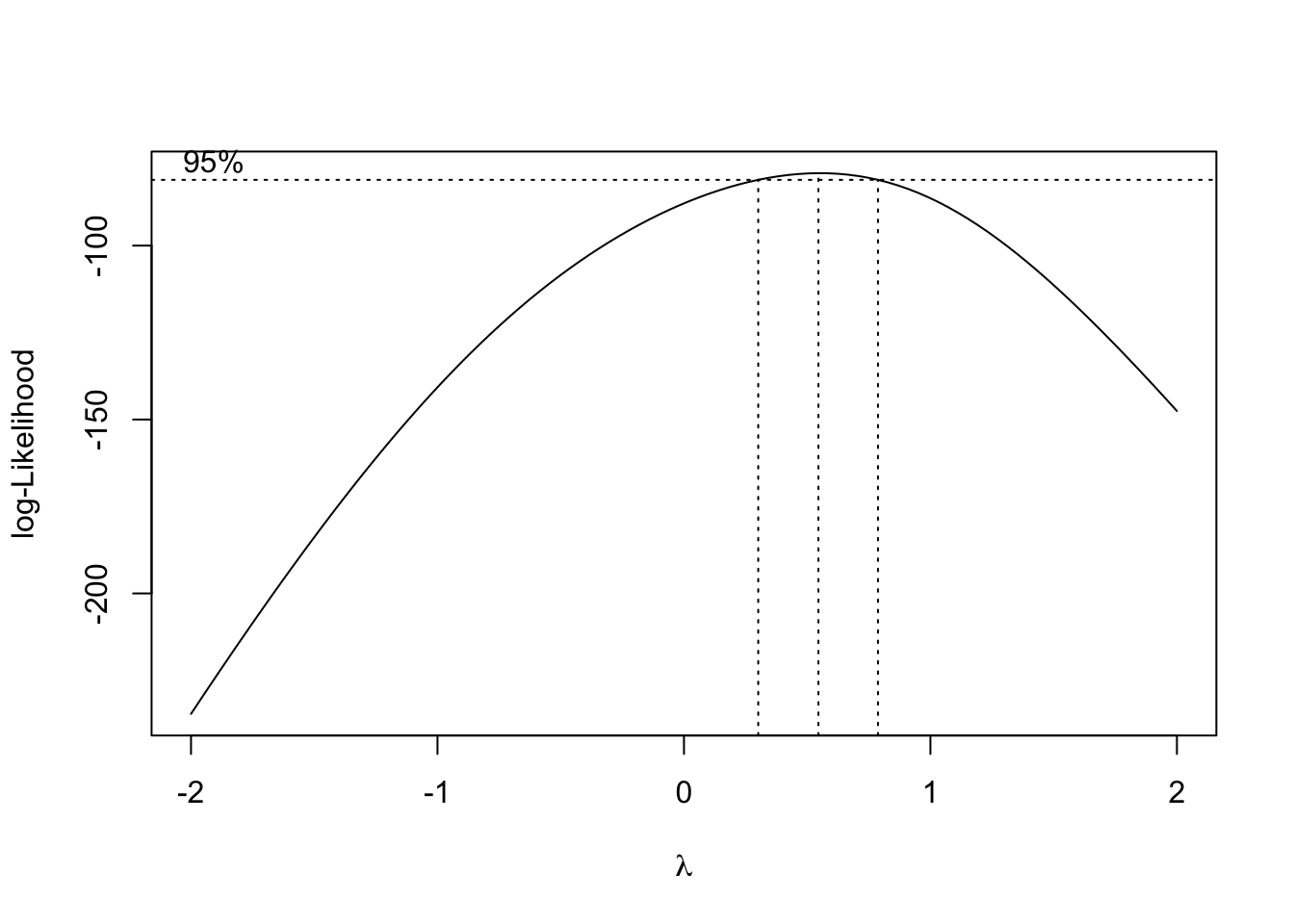
Example 5.3 : The Electric Utility Data
We use the Box-Cox procedure to select a variance-stabilizing transformation. The values of \(SS_{Res}(\lambda)\) for various values are shown in the table ..
boxcoxResult = boxcox(ex51$y_.kW. ~ ex51$x_.kWh., data = ex51, lambda = seq(-2,2,0.125))